1 Introduction
1.1 Role of Extreme Value Theory
Consider a set of observations from independent and identically distributed (IID) random variables \(X_1, \ldots, X_n\), with an unknown distribution function \(F\).
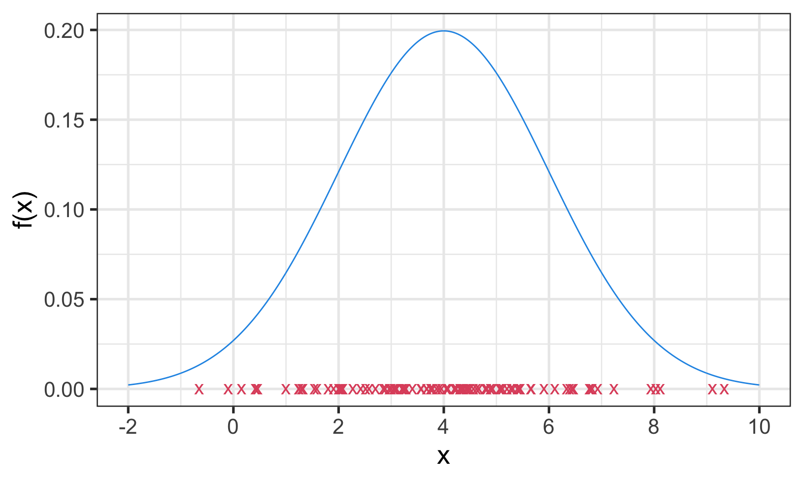
Figure 1.1: Data density
Suppose we want to estimate the tails of \(F\). Figure 1.1 illustrates the difficulties of estimating the tails of \(F\) accurately:
- most data are concentrated towards the centre of the distribution;
- by definition observations in the tails are scarce;
- estimates are often required beyond the sample maxima or minima;
- estimation is going to be difficult and will be driven strongly by the assumptions made.
1.1.1 Inadequacies of standard statistical approaches
Why can standard modelling approaches not be used for estimating tails?
We could fit a distributional model, e.g. \(N(\mu,\sigma^2)\), to all the data available and use this model to estimate tail probabilities; \[\begin{align*} \hat{\Pr}(X>x)=1-\hat{F}(x) =1-\Phi\left(\frac{x-\hat{\mu}}{\hat{\sigma}}\right) \end{align*}\] Problems with this include:
- estimates of \(\mu\) and \(\sigma\) are primarily driven by the central values of the data;
- assessment of model fit is driven by the central values;
- different models that fit the body of the data well can have very different extrapolations;
- if interest is only in the tails, why compromise the fit there by attempting to model the body of the distribution simultaneously?
Extreme value theory provides procedures for tail estimation which are scientifically and statistically rational. It is also intrinsically about extrapolation.
- in all undergraduate courses we are taught not to trust any extrapolation (usually in regression contexts);
- in many applications extrapolations are necessary, so it seems sensible to develop procedures that have some scientific basis.
1.2 Application areas of extreme value theory
In the course we will see a range of examples. In general, the most active areas of application of extreme value theory are (in order of activity):
- Environment (sea-levels, river-levels, wind speeds, temperatures, rainfall, pollution concentrations);
- Finance (financial markets, investment returns, insurance/re-insurance liabilities, actuarial lifetimes, portfolio risk)
- Internet traffic (file size, number and duration of connections);
- Reliability (weakest link principle)
- Athletics
- Statistical inference/tests. e.g. inference for \(\theta\) when \(X_i\sim U(0, \theta)\) for \(i=1, \ldots, n\). MLE \(\hat{\theta}\) satisfies: \[\begin{align*} \hat{\theta}=\max(X_1, \ldots, X_n). \end{align*}\]
- Asymptotic theory for sums.
1.2.1 Oxford and Worthing annual maxima temperatures
The first data set, shown in Figure 1.2, gives measurements of annual maxima temperatures in degrees Fahrenheit from 1901 to 1980 in Oxford and Worthing, England.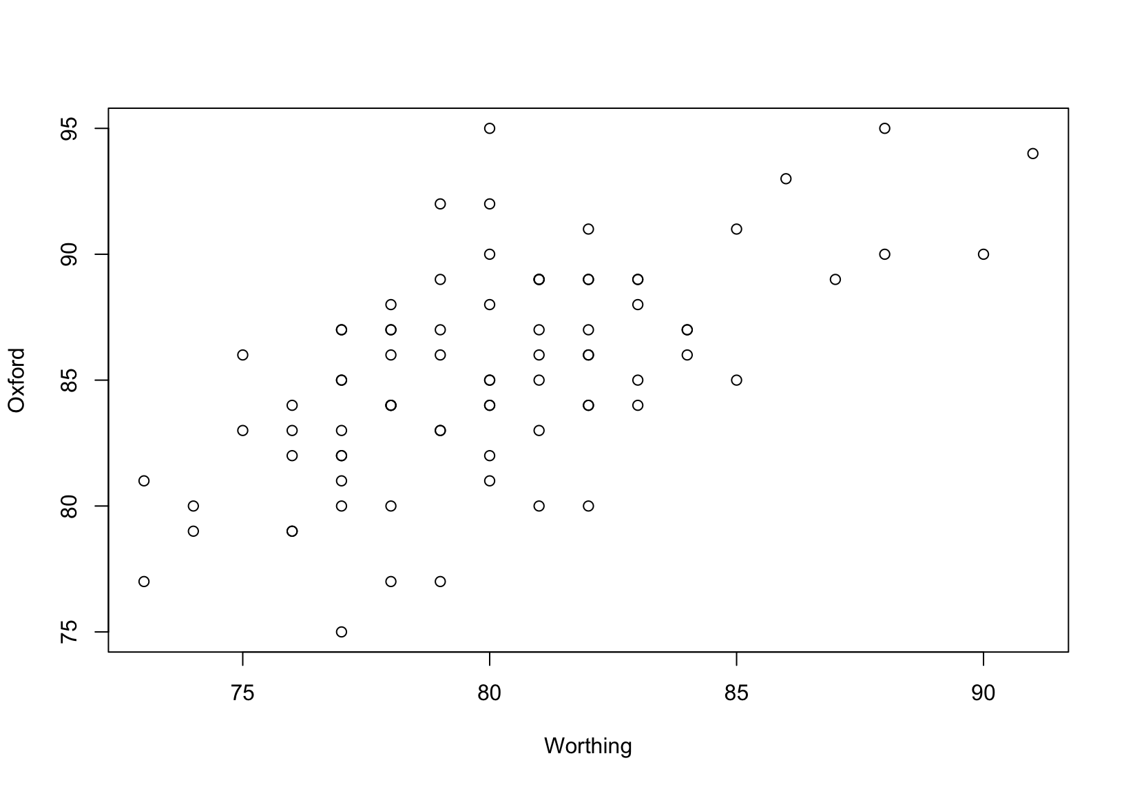
Figure 1.2: Annual maximum temperatures at Oxford and Worthing.
1.2.2 Oceanographic variables
Figure 1.3 shows concurrent measurements of two oceanographic variables taken just off the Cornish coast at Newlyn:
- Surge (m): the non-tidal component of still water height, driven by local pressure systems and by wind;
- Wave height (m): also driven by wind and local meteorological conditions.
In this example, dependence is due to reliance on common covariates.
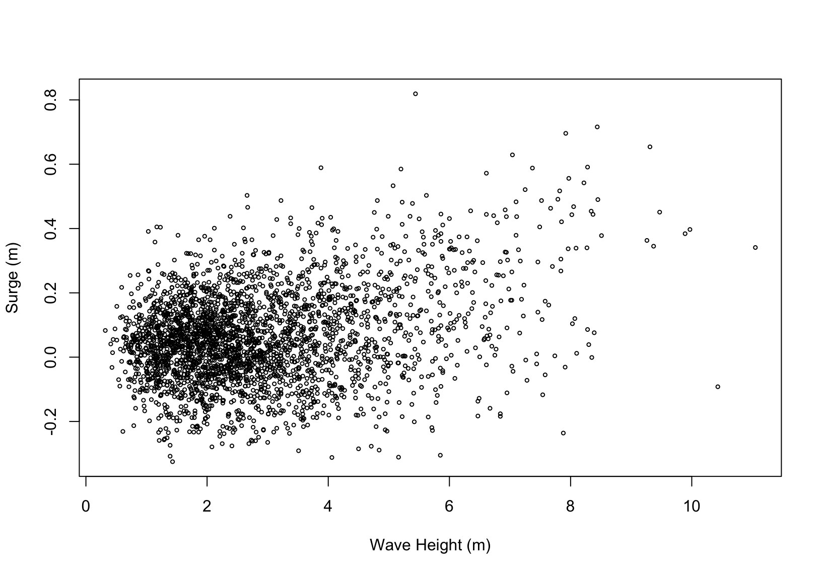
Figure 1.3: Surge and wave height at Newlyn.
1.2.3 FTSE Index
THE FTSE100 index of the top UK 100 shares in an established index of share price with many investment portfolios set up to track its movement. Figure 1.4 shows data on the end of day value of the FTSE index on each week day over the period 1968 to 2001.
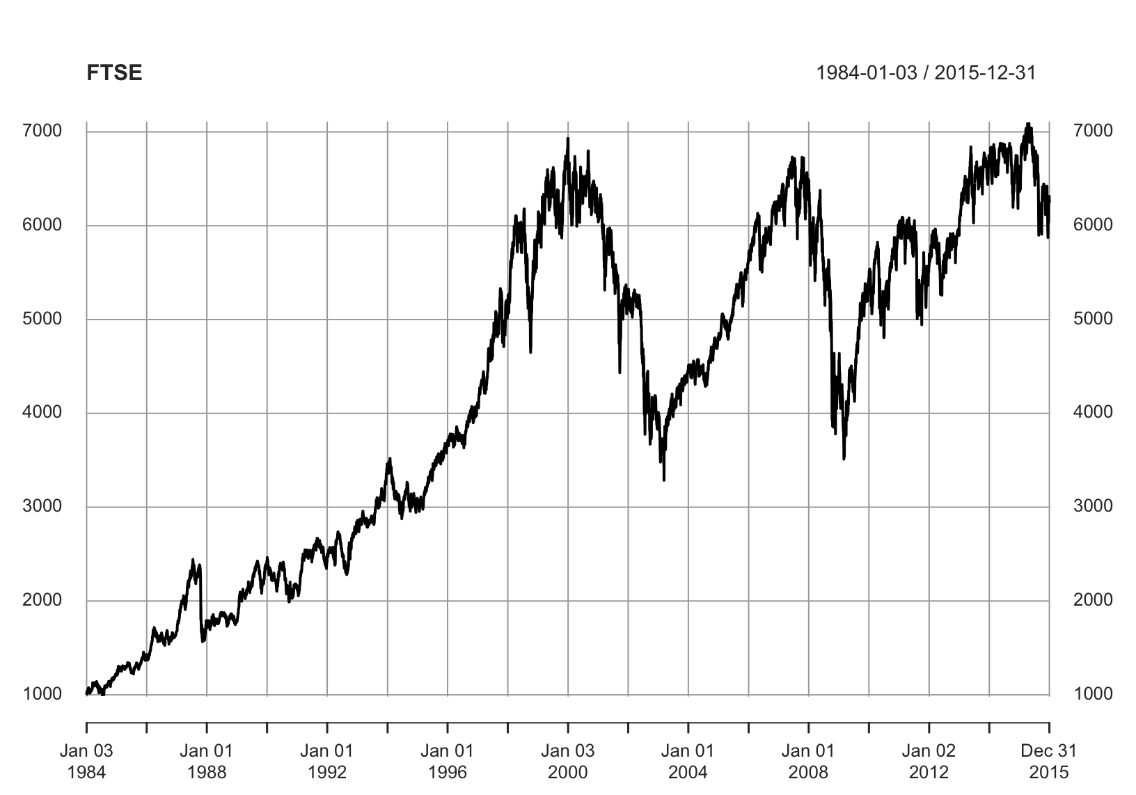
Figure 1.4: Time-series of FTSE100 index.
The general pattern in exponential growth, with some noticeable drops in value corresponding to the Stock Market crashes of Black Monday in October 1987, the Asian crash in 1999 and the reaction to 2001-09-11.
The index value on a given day is highly related to the value the day before. However, what is interesting to the investor is how it changes from one day to the next, relative to its current value. These relative changes are given by the new variables \[\begin{align*} X_t=\frac{FTSE_t-FTSE_{t-1}}{FTSE_{t-1}}\quad\mbox{ for each } t, t=2,3,\ldots \end{align*}\] which we term the returns, plotted in Figure 1.5. The average value of the returns series is much more stable over time.
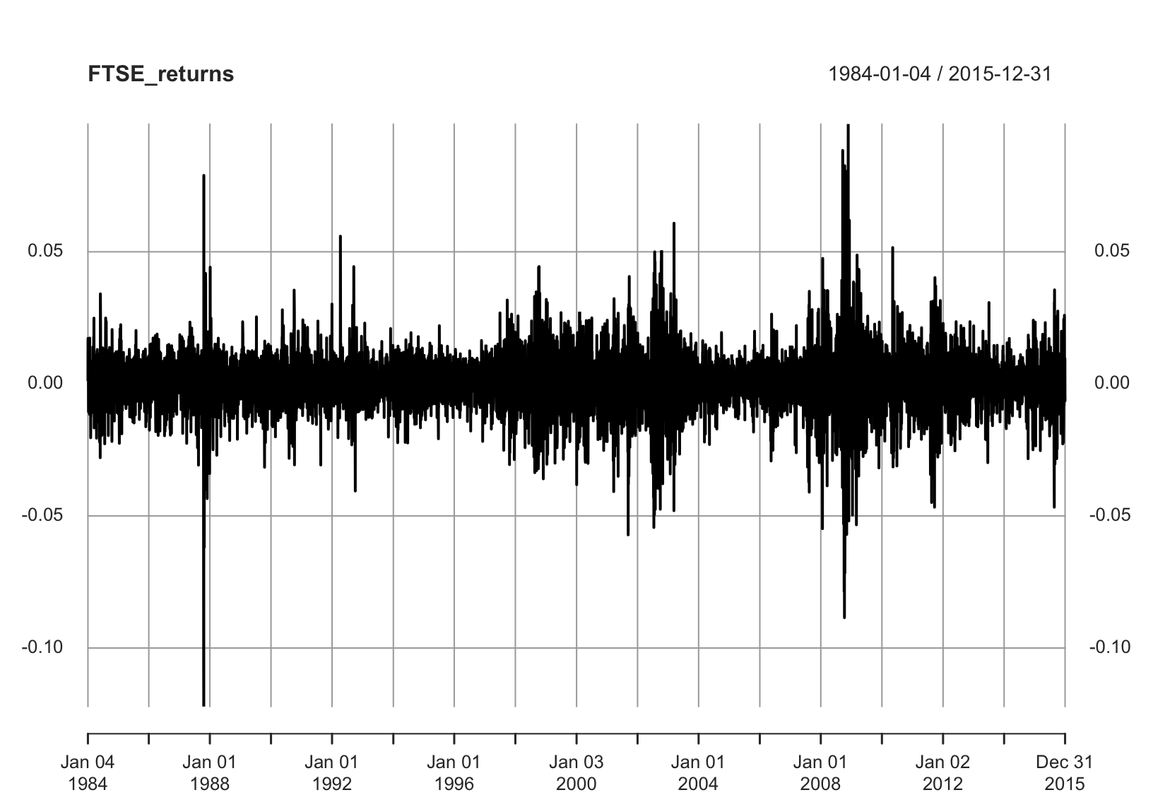
Figure 1.5: Time-series of FTSE returns.
1.3 What’s in the course for you?
This course will give you:
- an appreciation for a formal strategy for statistical modelling;
- insight into the issues associated with using asymptotically motivated models;
- an awareness of an area of probability theory rarely studied at undergraduate level;
- practice in applying standard statistical inference techniques in a new area of statistical application; and
- more background in the CLT and point / Poisson processes.