6 Statistical Inference for Extremes of Stationary Processes
We now consider the additional practical difficulties encountered due to dependence in analysing the extreme values of a stationary process. In a practical data analysis we have to:
- select a high threshold;
- identify clusters of extreme values which are independent from one another;
- estimate the extremal index;
When clusters are defined we
- extract the cluster maxima and fit the GPD distribution to the cluster maxima over the threshold;
- estimate characteristics of the cluster;
- assess sensitivity of cluster characteristics to threshold selection.
6.1 Identifying independent clusters
There are a number of ways of identifying independent clusters of extreme values. Here we will focus on the runs method, proposed by Smith and Weissman (1994), but blocks and intervals methods also exist (Ferro and Segers 2003), and Ledford and Tawn (2003) identified conditions that could be tested for independence between clusters.
6.1.1 The runs method: declustering
For a selected high threshold \(u\) we conclude that if consecutive exceedances of the threshold \(u\) are separated by a set of \(m\) consecutive observations below the threshold \(u\) then the exceedances belong to separate clusters.
Similarly, exceedances separated by less than \(m\) consecutive non-exceedances are deemed to be in the same cluster.
The choice of \(u\) and \(m\) is critical, \(m\) needs to be the time lag when the process is independent in the extremes.
The runs method: extremal index estimation
This algorithm motivates the runs estimator of the extremal index \(\theta\).
- Use the empirical form the extremal index, \[\begin{eqnarray*} \hat{\theta}(u,m) & = & \hat{\Pr}(M_{2,m+1}\leq u\,|\, X_1>u), \end{eqnarray*}\] using the empirical probability.
- \(\hat{\theta}(u,m)\) is identical to \(1/\mbox{mean cluster size}\) with clusters defined by the runs method.
Example: daily rainfall data
We illustrate the use of these cluster identification and extremal index estimation using a time series of daily rainfall accumulations at a location in south-west England, recorded during 1914-1962. This data set is shown in Figure 6.1. Note that the series is assumed to be stationary over this observation period.
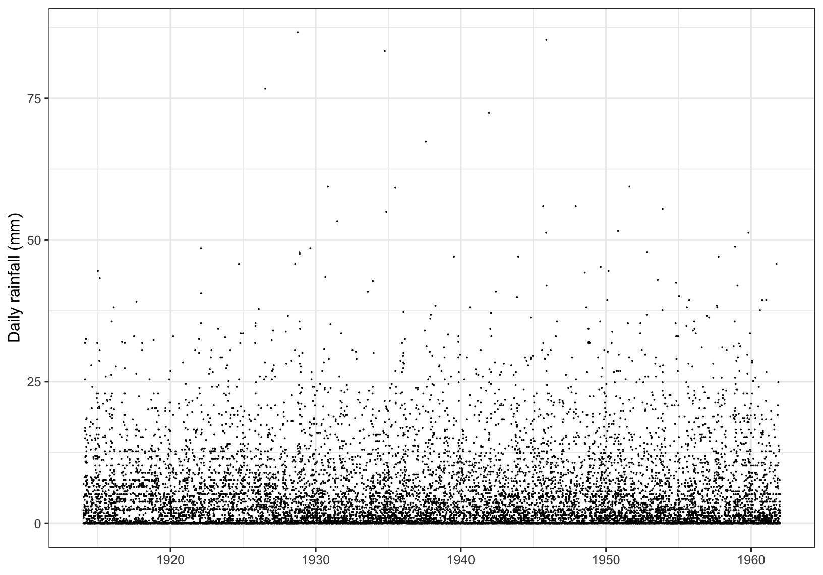
Figure 6.1: Daily rainfall.
Figure 6.2 shows a plot of the extremal index of the rainfall data, for \(m=1\) and \(m=2\). From this we can see that
- \(\hat{\theta}(u,m)\) are threshold dependent
- increasing \(m\) does not materially change our estimate \(\hat{\theta}(u,m)\)
- \(m=1\) is appropriate for cluster identification
- the value of \(\theta(u,m)\approx 1\) indicates weak short-range dependence with a limiting cluster size of 1 for higher thresholds.
- from experience we know rainfall episodes last a number of days, but this analysis tells us that extreme daily rainfall events tend to be isolated.
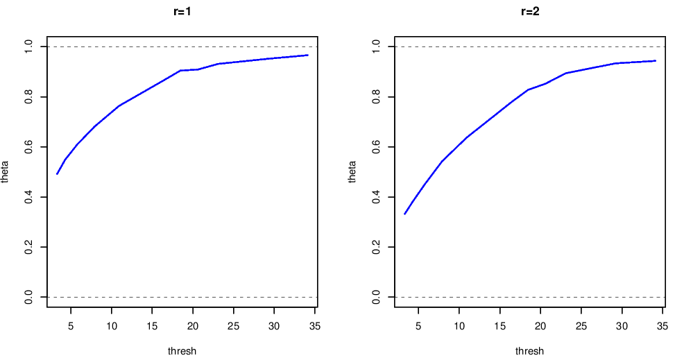
Figure 6.2: Extremal index estimates using the runs estimator with \(m=1\) or \(m=2\), for the rainfall data shown above.
Example: financial time series data
We now turn to estimating clustering for the financial time series data. We focus on the squared returns from the FTSE 100 share index; these are shown in Figure 6.3. We make the initial assumption that the series is stationary over this observation period. (Note: this is slightly different to the observation period shown in Figure 1.4.)
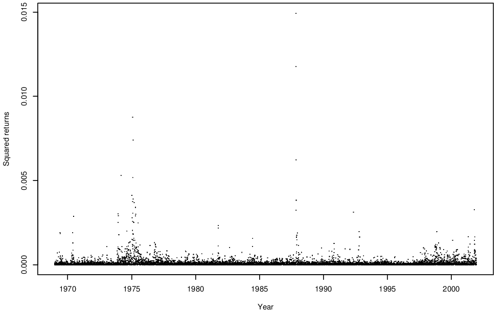
Figure 6.3: Squared returns for the FTSE 100 share index.
6.1.1.1 Extremal index for the squared FTSE returns
The extremal index for the squared returns shown in Figure 6.3 is shown in Figure 6.4. From this plot we can see that
- \(\hat{\theta}(u,m)\) is stable for \(u\geq 0.005\) corresponding to the 0.95 quantile of the squared returns;
- the value of \(\hat{\theta}(u,m)\approx0.35\) suggests that the mean cluster size is around 2.9;
- \(m=10\) seems fine for cluster identification.
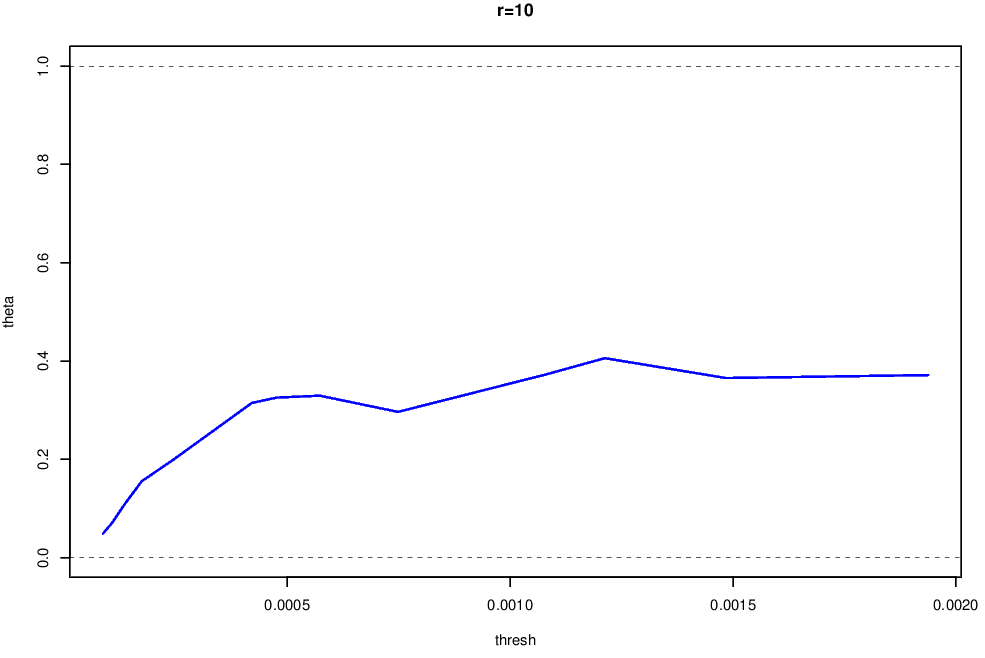
Figure 6.4: Extremal Index of the squared returnes for the FTSE 100 data, estimated using the runs method with \(m=10\).
We now investigate the source of serial dependence being the changing volatility of the process. We first standardise the returns series by
- subtracting the local mean
- dividing by the local standard deviation
We work with the squared standardised series as shown in Figure 6.5. Local means and standard deviations were calculated using the \(h=20\) observations centred on the value to be standardised. There is little sensitivity to this choice of \(m\) for values of \(h\) between 2 and 50.
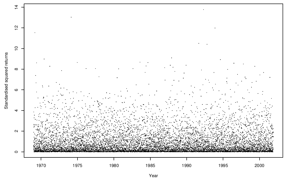
Figure 6.5: Standardised squared returns for the FTSE 100 series.
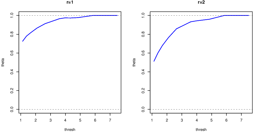
Figure 6.6: Extremal index for the standardised squared returns of the FTSE 100 series. Estimates made using the runs method with \(m=1\) and \(m=2\).
The extremal index for the squared standardised returns is shown in Figure 6.6. From this plot,
- estimates of \(\theta(u,m)\) are threshold dependent;
- increasing \(m\) does not materially change our conclusions, \(m=1\) is fine for cluster identification;
- the limiting value of \(\theta=1\) indicates weak short-range independence with a limiting cluster size of 1;
- by undertaking the more sophisticated analysis and standardising the series we appear to have accounted for all the short-range dependence in the series.
6.2 Modelling cluster maxima and all exceedances
For a specific threshold \(u\), we can
- model the cluster maxima
- fit the GPD\((\sigma_u,\xi)\) model for cluster maxima excesses over \(u\).
- standard errors can be obtained by usual methods as cluster maxima are independent.
- model all exceedances
- fit the GPD\((\sigma_u,\xi)\) model for the excess of all exceedances over \(u\).
- the data are dependent so block bootstrap methods are needed for standard error evaluation.
6.2.1 Point process intensity estimation
To estimate \(\mu\) and \(\sigma\) in the point process intensity we need information in addition to that given by our estimate of \(\sigma_u\) and \(\xi\). This information is given by the expected number of cluster maxima exceeding \(u\). Equating the point process and sample values gives \[\begin{eqnarray*} \theta [1+\xi(u-\mu)/\sigma]_+^{-1/\xi}=n_{cl,u}. \end{eqnarray*}\] It follows that \[\begin{eqnarray*} \hat{\sigma}=\hat\sigma_u(n_{exc,u})^{\hat{\xi}}\mbox{ and } \hat{\mu}=u+(\hat{\sigma}-\hat{\sigma}_u)/\hat{\xi}. \end{eqnarray*}\]
Note that \(\theta\) is estimated by \(\hat{\theta}_u =n_{cl,u}/n_{exc,u}\), i.e. the number of clusters above \(u\) divided by the number of exceedances of \(u\).
Example: Squared FTSE returns
For the squared FTSE returns
- using a declustering parameter of \(m=10\) and a threshold of \(u=0.004\) corresponding to the 0.95 quantile of the squared returns gives \(n_{cl,u}=134\) independent clusters
- there are \(n_{exc,u}=429\) exceedances of \(u\)
- we estimate the extremal index as \(\hat\theta=0.31\)
- fitting a GPD to cluster maxima gives \[\begin{eqnarray*} \hat\sigma_u = 0.000232 (0.0000679) ~~~\hat\xi = 0.653 (0.152) \end{eqnarray*}\]
- combining the above estimates gives \[\begin{eqnarray*} \hat{\sigma}=\hat\sigma_u(n_{exc,u})^{\hat{\xi}} = 0.012\mbox{ and } \hat{\mu}=u+(\hat{\sigma}-\hat\sigma_u)/\hat{\xi} = 0.0223. \end{eqnarray*}\]