3 Alternative Characterisation and Improved Inferences
So far, our interest has been in extreme values and asymptotically motivated models for tail estimation of \(F\) (the distribution of \(X\)). We have focused on asymptotic models for \(G\), the distribution of normalised \(M_n\). With regard to our objective this is
- not directly relevant theoretically, and
- likely to lead to inefficient statistical procedures - see Figure 3.1.
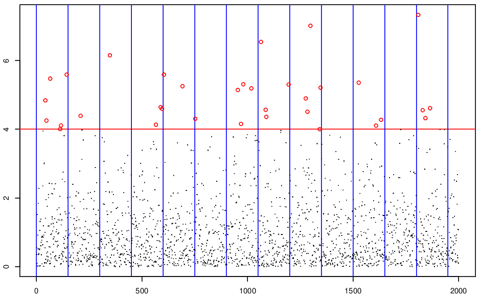
Figure 3.1: Peaks over threshold v. block maxima.
Motivation for extension of theory for maxima
We want to learn about possible asymptotically motivated models for \(F\) arising from the limiting distribution \(G\). We will initially follow a heuristic approach making approximations that we will subsequently justify rigorously.
Assume that the limit representation holds for some large \(n\); this means that \[\begin{eqnarray} \{F(a_n x+b_n)\}^n \approx G(x)=\exp\left[-(1+\xi x)_+^{-1/\xi}\right], \tag{3.1} \end{eqnarray}\] for all \(x\) such that \(a_n x+b_n\) is near \(x^F\). Specifically assume that there is a threshold \(u\) near \(x^F\) such that equation (3.1) holds for all \(x\) with \(a_n x+b_n>u\).
From equation (3.1) it follows that \[\begin{eqnarray*} F(a_n x+ b_n) & \approx & G^{1/n}(x) \mbox{ for }a_n x+b_n>u\\ F(y) & \approx & G^{1/n}\left( \frac{y-b_n}{a_n}\right) \mbox{ for }y>u.\\ \end{eqnarray*}\] The RHS here is still a GEV distribution due to the max-stability property. Hence for some \(\mu, \sigma>0, \xi\) parameters \[\begin{eqnarray*} F(y) & \approx & \exp\left[-\left\{1+\xi\left(\frac{y-\mu}{\sigma}\right) \right\}_+^{-1/\xi}\right]\mbox{ for }y>u\\ F(y) & \approx & 1-\left[1+\xi\left(\frac{y-\mu}{\sigma}\right) \right]_+^{-1/\xi}\mbox{ for }y>u. \end{eqnarray*}\] This approximation is like a tail expansion for \(F\) near \(x^F\), with the tail corresponding to the upper tail of a GEV distribution.
We will also focus on the distribution of the exceedances of a high threshold, i.e. \(X\,|\,X>u\). Alternatively we may define the excess of threshold \(u\) as \[\begin{eqnarray*} Y_u=(X-u)_+. \end{eqnarray*}\] Then for \(y\geq 0\) \[\begin{eqnarray} \Pr(Y_u>y\,|\,Y_u>0) & = & \Pr(X>u+y\,|\, X>u)\nonumber\\ & = & \frac{1-F(u+y)}{1-F(u)}\nonumber\\ & \approx & \frac{[1+\xi(u+y-\mu)/\sigma]_+^{-1/\xi}} {[1+\xi(u-\mu)/\sigma]_+^{-1/\xi}}\nonumber\\ & = & [1+\xi y/\sigma_u]_+^{-1/\xi}, \label{eqn:gpd} \end{eqnarray}\] where \(\sigma_u=\sigma+\xi(u-\mu)\). It follows that \(Y_u\,|\,Y_u>0\sim \mbox{GPD}(\sigma_u,\xi)\), i.e. a generalised Pareto distribution with scale parameter \(\sigma_u\) and shape parameter \(\xi\).
In general, if \(Y \sim \mbox{GPD}(\sigma, \xi)\), the cumulative distribution function is given by \[ F(y) = \left\{\begin{array}{ll} 1 - \left(1 + \xi\frac{y}{\sigma}\right)^{-1/\xi}, & \mbox{ for } \xi \neq 0, y>0, 1 + \xi\frac{y}{\sigma}>0, \\ 1 - \exp\left(-\frac{y}{\sigma}\right) & \mbox{ for } \xi=0, y>0. \end{array}\right. \]
3.1 Point process characterisation
Assume that
- \(X_1, \ldots ,X_n\) are IID with distribution function \(F\);
- \(F\) is in the domain of attraction of \(G\) a GEV\((0,1,\xi)\) distribution;
- the required norming constants are \(a_n\) and \(b_n\).
We construct a sequence of point processes \(P_1, P_2, \ldots\) on \([0,1]\times [0,\infty)\) by \[\begin{eqnarray*} P_n=\left\{\left(\frac{i}{n+1},\frac{X_i-b_n}{a_n}\right);i=1, \ldots ,n \right\} \end{eqnarray*}\] and examine the limit process.
Figure 3.2 shows examples of point process \(P_n\) for \(n=5,10,100,500,1000,10000\) respectively with \(X_i\sim\) Exp(1).
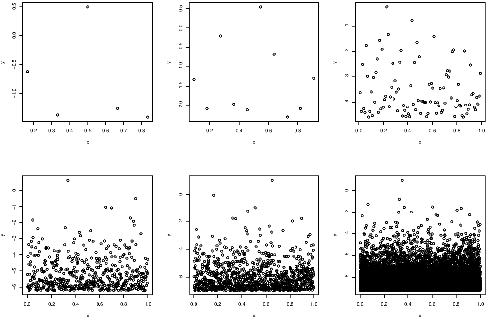
Figure 3.2: Example of point processes of various lengths.
Notes on point process convergence:
- the limit process is non-degenerate as \((M_n-b_n)/a_n\) (which is the largest point in the \(y\)-axis) is non-degenerate;
- small points are normalised to the same value \(b_l\), with \[\begin{eqnarray*} b_l=\lim_{n\rightarrow \infty}\frac{x_F-b_n}{a_n}; \end{eqnarray*}\]
- large points of the process are retained in the limit process;
- if we can describe the limit process we have an asymptotically motivated model for all large values.
3.1.1 Aside on Poisson processes
Consider a non-homogeneous Poisson process with intensity \(\lambda(x)\) on the set \(C\). Let \(N(A)\) be the number of points of the Poisson process in the set \(A\subset C\). The process then has the following properties:
- \(N(A)\) is a Poisson random variable for any \(A\subset C\);
- The expected value of \(N(A)\) is obtained by integrating the intensity: \[\begin{eqnarray*} E(N(A))=\int_{x\in A} \lambda(x)dx=\Lambda(A), \end{eqnarray*}\] where \(\Lambda(A)\) is termed the integrated intensity;
- \(N(B_1), \ldots ,N(B_k)\) are independent random variables for any \(k\) and any disjoint sets \(B_1, \ldots ,B_k\), with \(B_i\subset C\) for all \(i\);
- The location of points of \(A\) have density \(\lambda(x)/\Lambda(A), x\in A\).
3.1.2 The limiting point process
Theorem
Under the above condition on \(P_n\), on the set \([0,1]\times (b_l+\epsilon,\infty)\), where \(\epsilon>0\),
\[\begin{eqnarray*}
P_n \rightarrow P \mbox{ as }n\rightarrow \infty,
\end{eqnarray*}\]
where \(P\) is a non-homogeneous Poisson process with intensity
\[\begin{eqnarray*}
\lambda(t,x)=(1+\xi x)_{+}^{-1-1/\xi}.
\end{eqnarray*}\]
We will often be interested in sets of the form \[\begin{eqnarray*} B_y=[0,1]\times (y,\infty) \end{eqnarray*}\] where \(y>b_l\), for which \[\begin{eqnarray*} \Lambda(B_y) & = & \Lambda([0,1]\times (y,\infty))\\ & = & \int_{t=0}^{1} \int_{x=y}^{\infty}\lambda(t,x)\,dxdt\\ & = & \int_{t=0}^{1} [-(1+\xi x)_{+}^{-1/\xi}]_{x=y}^{\infty}\,dt\\ & = & \int_{t=0}^{1} (1+\xi y)_{+}^{-1/\xi} \,dt\\ & = & (1+\xi y)_{+}^{-1/\xi}. \end{eqnarray*}\]
3.1.3 Proof of point process limit
The strategy for proving that a point process \(P_n\) converges to a limit process \(P\) is as follows (Kallenberg 1983).
Let \(N_n(B)\) and \(N(B)\) be the number of points of \(P_n\) and \(P\) respectively in set \(B\). Then for unions of sets of the form \[\begin{eqnarray*} B=(c_1,d_1]\times \ldots \times (c_m,d_m] \end{eqnarray*}\] we have to show that as \(n\rightarrow \infty\) \[\begin{eqnarray*} E(N_n(B))\rightarrow E(N(B)) \end{eqnarray*}\] and \[\begin{eqnarray*} \Pr(N_n(B)=0)\rightarrow \Pr(N(B)=0). \end{eqnarray*}\]
Proof of Limit
Take \(B_y=(0,1]\times (y,\infty)\)
The \(i\)-th point of \(P_n\) is in \(B_y\) if \[\begin{eqnarray*} \frac{X_i-b_n}{a_n}>y \mbox{ i.e. if }X_i>a_n y +b_n \end{eqnarray*}\]
The probability of this is \(1-F(a_n y +b_n)\). Thus the expected number of such points is \[\begin{eqnarray*} E(N_n(B_y)) & = & n[1-F(a_n y +b_n)]\\ & \sim & -\log \{F(a_n y +b_n)\}^n\\ & \rightarrow & -\log G(y)\\ & = &(1+\xi y)_{+}^{-1/\xi}\\ & = & \Lambda([0,1]\times (y,\infty))\\ & = & \Lambda(B_y)\\ & = & E(N(B_y)). \end{eqnarray*}\]
Now consider the event \(N_n(B_y)=0\). This can be expressed as \[\begin{eqnarray*} \{N_n(B_y)=0\}= \left\{\frac{X_i-b_n}{a_n}\leq y ~~\forall i=1, \ldots ,n\right\} =\left\{X_i \leq a_ny+b_n ~~\forall i=1, \ldots ,n\right\} \end{eqnarray*}\] So \[\begin{eqnarray*} \Pr(N_n(B_y)=0) & = & \{F(a_n y+b_n)\}^n\\ & \rightarrow & G(y)\\ & = & \exp[-(1+\xi y)_{+}^{-1/\xi}]\\ & = & \exp[-\Lambda(B_y)]\\ & = & \Pr(N(B_y)=0). \end{eqnarray*}\]
3.1.4 The value of the Poisson process limit
- The result shows that the behaviour of all large values is determined (asymptotically) by the \(a_n, b_n\) and \(\xi\) characteristics (just as for the maximum);
- if we use all threshold exceedances for statistical inference we have more data to use for inference but the same number of parameters to estimate as using maxima, this suggests potential efficiency gains;
- the likelihood for a Poisson process observed on \([0,1]\times (u,\infty)\) applied to exceedances \((t_1, x_1), \ldots ,(t_{n_u},x_{n_u})\}\) of \(u\) is \[\begin{eqnarray} \prod_{i=1}^{n_{u}}\lambda(t_i,x_i) \times \exp\{-\Lambda([0,1]\times (u,\infty))\}. \tag{3.2} \end{eqnarray}\] See Smith (1989) for statistical details of the point process approach.
3.2 Threshold exceedances
An important consequence of the Poisson process result is that it provides an asymptotic motivation for the generalised Pareto distribution as a conditional model for excesses of a high threshold.
We focus on points of the process \(P_n\) that are large i.e. above a threshold) and look at the distribution of exceedances of this level. For any fixed \(v>b_l\), let \[\begin{eqnarray*} u_n(v)=a_n v+b_n, \end{eqnarray*}\] then \(u_n(v)\rightarrow x^F\), and let \(x>0\) then \[\begin{align*} &\Pr(X_i>a_n x+u_n(v)\,|\, X_i>u_n(v))\\ &\quad=\Pr\left(\frac{X_i-b_n}{a_n}>x+v \,\left |\,\frac{X_i-b_n}{a_n}>v\right. \right)\\ &\quad=\Pr\left(\mbox{a given point in } P_n>x+v \,|\, \mbox{a given point in } P_n>v\right)\\ &\quad \rightarrow \Pr\left(\mbox{a given point in } P>x+v \,|\, \mbox{a given point in } P>v\right)\\ &\quad= \frac{\Lambda(B_{x+v})}{\Lambda(B_{v})}\\ &\quad= \left[1+\xi\frac{x}{1+\xi v}\right]_+^{-1/\xi}\\ &\quad= \left[1+\xi\frac{x}{\sigma_v}\right]_+^{-1/\xi}, \end{align*}\] where \(\sigma_v=1+\xi v\).
Hence the limiting distribution for a scaled excess \[\begin{eqnarray*} \frac{[X_i-u_n(v)]_+}{a_n}\,|\,X_i>u_n(v) \end{eqnarray*}\] follows a generalised Pareto distribution, GPD\((\sigma_v,\xi)\).
Threshold Stability:
Furthermore, this limit distribution holds whatever value of \(v\), provided \(v>b_l\). Hence there is stability of the form of the limit distribution with respect to the level of the threshold, provided the threshold is large enough for the Poisson process limit to be achieved.
3.2.1 Practical implications of limit
This limiting result motivates the use of the GPD as a model for excess values over a threshold. This requires fixing \(u_n(v)\) at a high threshold, absorbing \(a_n\) into the scale parameter and taking the limit as an equality for all \(x>0\). Let \(Y_u\) be the excess variable over threshold \(u\): \[\begin{eqnarray*} Y_u =(X-u)_+ \end{eqnarray*}\] then for \(y>0\) \[\begin{eqnarray*} \Pr(Y_u\leq y\,|\,Y_u>0)=1-(1+\xi y/\sigma_u)_+^{-1/\xi} \end{eqnarray*}\] so \(Y_u\,|Y_u>0\sim \mbox{GPD}(\sigma_u,\xi)\).
We now have a model for the excess variable, conditional on having observed an excess. To undo this conditioning and obtain a model for the original variable \(X\) we model the rate parameter \[\begin{eqnarray*} \phi_u = \Pr(Y_u>0) = \Pr(X>u). \end{eqnarray*}\]
In the IID case, it follows from the Poisson process limit that the estimate for this is simply the proportion of the data which exceed \(u\) \[\begin{eqnarray*} \phi_u = \frac{n_u}{n} \end{eqnarray*}\] where \(n_u=\sum_{i=1}^n I[y_t>u]\) and \(I[y_t>u]\) is the indicator variable taking the value 1 if the observation is an exceedance.
3.2.2 Properties of GPD
Influence of shape parameter
As with the GEV, the parameter \(\xi\) has a substantial impact on the upper tail.
- \(\xi>0\) is heavy tailed;
- \(\xi=0\) is the Exponential distribution with mean \(\sigma_u\);
- \(\xi<0\) is short tailed, with upper bound.
Moments
For \(r<1/\xi\)
\[\begin{eqnarray*}
E(Y_u^r\,|\,Y_u>0)=\frac{\sigma_u}{\xi}\sum_{j=0}^r\binom{r}{j}
\frac{(-1)^{j+1}}{(1-\xi j)}
\end{eqnarray*}\]
otherwise
\[\begin{eqnarray*}
E(Y_u^r\,|\,Y_u>0)=\infty.
\end{eqnarray*}\]
More details of the GPD are given by Davison and Smith (1990).
3.2.3 Inference for the generalised Pareto distribution
The generalised Pareto distribution (GPD) is used to model data arising as independent threshold exceedances.
We assume that excesses \(Y_{u,1},\ldots,Y_{u,n}\) of a high threshold \(u\) follow GPD(\(\sigma,\xi\)) so that \[\begin{eqnarray*} \Pr(Y_u<y\,|\,Y_u>0)=1-\left\{1+\xi\left(\frac{y}{\sigma_u}\right)\right\}_+^{-1/\xi}~~~y>0. \end{eqnarray*}\]
Possibly the most important issue in statistical modelling of threshold exceedance data is the choice of threshold \(u\).
- Using as low a threshold as possible maximises the amount of data used, making the statistical inference more efficient;
- If too low a threshold is used, the GPD may not fit well as the asymptotic argument motivating its appropriateness may not apply.
A threshold choice based on the observed sample is required to balance these two opposing demands. We can exploit some properties of the GPD to help us with threshold selection.
Threshold stability
This property states that if the random variable \(Y_u\) satisfies
\[\begin{eqnarray}
Y_u\,|\,Y_u>0\sim\mbox{ GPD}(\sigma_u,\xi)\mbox{ for some threshold }u
\tag{3.3}
\end{eqnarray}\]
then for any higher threshold \(v\ge u\)
\[\begin{eqnarray*}
Y_v\,|\,Y_v>0 \sim\mbox{ GPD}(\sigma_u+\xi(v-u),\xi)
\end{eqnarray*}\]
so that \(\xi\) is constant with threshold but \(\sigma_v=\sigma_u+\xi(v-u)\) is not.
Linear mean excess
When \(Y_u\) satisfies (3.3), the mean excess over \(v>u\) is
\[\begin{eqnarray}
E(Y_u | Y_u>0) = \{\sigma_u + \xi(v-u)\}/(1-\xi),\mbox{ for }\xi<1.
\end{eqnarray}\]
Thus the shape parameter is invariant to threshold and \(E(Y_u| Y_u>0)\) is linear in \(v\) with gradient \(\xi/(1-\xi)\).
Formal algorithms that use within-sample characteristics to select a threshold by minimising the mean square error of the estimated shape parameter, under certain assumptions about the second order tail structure, have been proposed (Danielsson and Vries 1997; Guillou and Hall 2001).
Threshold selection diagnostics: Mean excess (or residual life) plot
The sample mean excess over a threshold is plotted against the threshold, for a range of threshold values. If the random variable follows a generalised Pareto distribution over a threshold \(u\) then the relationship shown by the plot should be a straight line above \(u\) with gradient \(\xi/(1-\xi)\). Confidence intervals are added to each of these plots using the approximate Normality of sample means.
Threshold selection diagnostics: Parameter stability plot
We re-parameterise the threshold dependent scale parameter \(\sigma_v\) given above as follows:
\[\begin{eqnarray}
\sigma^\ast=\sigma_v-\xi v
\end{eqnarray}\]
Now \(\sigma^\ast\) does not depend on the choice of \(v\), provided the original threshold for fitting (\(u\)) is high enough.
The estimated parameters \(\hat\sigma^\ast\) and \(\hat\xi\) are plotted against the threshold used for estimation. If the random variable follows a generalised Pareto distribution over a threshold \(u\) then both parameters \((\sigma^\ast,\xi)\) will be constant for exceedances of all thresholds \(v\) greater than \(u\). The selected threshold corresponds to the lowest value for which the described properties are achieved. Again, confidence intervals are added to this plot using the approximate Normality of the maximum likelihood estimates of the parameters.
3.2.4 Example: fitting the GPD to Newlyn data
Note: The points made in Section 2.3.1 concerning maximum likelihood for the GEV distribution all apply equally to the use of maximum likelihood to fit the GPD to threshold exceedance data.
In order to fit the GPD to the Newlyn wave and surge data, we must first choose an appropriate threshold. The mean residual life plots for these data sets are shown in Figure 3.3. These plots suggest a threshold of at least 0.05 for the surge and at least 1.5 for the waves.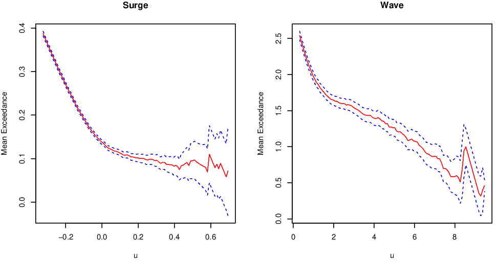
Figure 3.3: Mean excess plots for the Newlyn surge and wave data sets.
Parameter stability plots for the surge variable are shown in Figure 3.4, and for the wave height variable in Figure 3.5. For surge, the parameter stability plots suggest a threshold of at least 0.1. For the wave variable, the parameter stability plots suggest a threshold of at least 2.
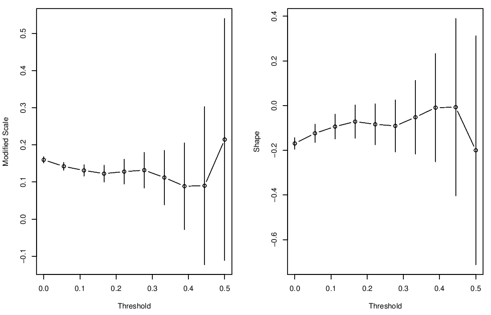
Figure 3.4: Parameter stability plots for the Newlyn surge variable.
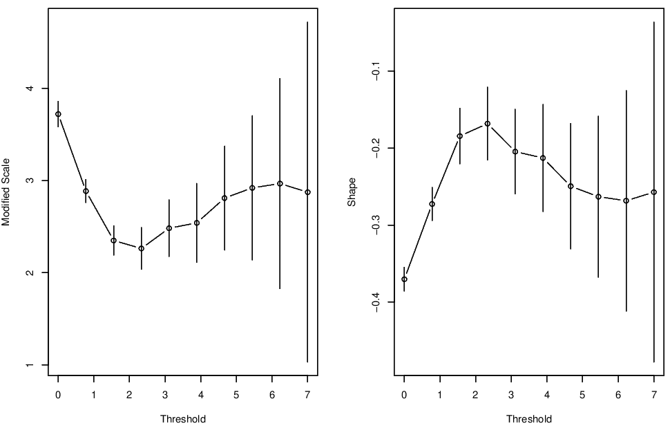
Figure 3.5: Parameter stability plots for the Newlyn wave variable.
We proceed with thresholds of 0.1 and 2 for the surge and wave respectively. These correspond to the 0.64 and 0.353 quantiles of these variables respectively.
Parameter estimates for the GPD fitted at these thresholds are:
| Surge | Wave | |
|---|---|---|
| \(\hat\sigma\) | 0.12 (0.005) | 1.91 (0.061) |
| \(\hat\xi\) | -0.10 (0.026) | -0.165 (0.022) |
| Corr\((\hat\sigma,\hat\xi)\) | -0.73 | -0.80 |
Both of these distributions are estimated to have a finite upper endpoint. Finally, Figure 3.6 displays contours of the log-likelihood surface showing the negative dependence between these parameters.
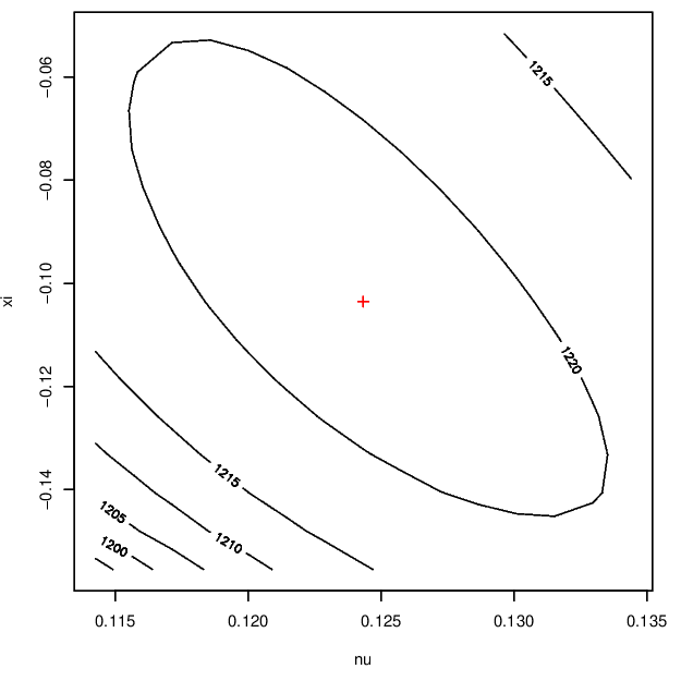
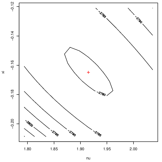
Figure 3.6: Log-likelihood surfaces for the GP parameter for Newlyn surge (left) and wave (right) data.
3.2.5 Q-Q plot & probability integral transform
One common diagnostic plot is the Q-Q plot, which shows the empirical quantiles (according to actual data) against the expected quantiles (according to the model). When fitting the GEV or the GPD, it is possible that a lot of the plotting space is taken up by the few largest values. The plot might be clearer on a different scale.
Transforming scales
The probability integral transform (PIT) tells us that if \(X\sim F\) then
\[\begin{eqnarray*}
U=F(X)\sim \mbox{Unif}(0,1)
\end{eqnarray*}\]
and if \(U \sim \mbox{Unif}(0,1)\) then
\[\begin{eqnarray*}
Y=G^{-1}(U) \sim G.
\end{eqnarray*}\]
Putting these two together, we get for \(Y_u=(X-u)_+ \sim\) GPD(\(\sigma_u, \xi\))
\[\begin{eqnarray*}
\frac{1}{\xi}\log\left[1+\xi\left(\frac{X-u}{\sigma_u}\right)\right] \sim \mbox{Exp}(1).
\end{eqnarray*}\]
This leads to a Q-Q plot on a transformed scale, by computing the empirical quantiles using the expression on the left hand side (with \(X\) substituted by the data points), and the theoretical quantiles according to the Exp\((1)\) distribution.
3.2.6 Return levels & return periods
To estimate the return level \(x_p\) corresponding to return periods \(1/p\), we need to solve \[ 1 - F(x_p) = p \,. \] For a given threshold \(u\), assume that \(\phi_u = \Pr(X>u)\). For practical interest, we assume that \(p\) is much smaller than \(\phi_u\).
As \(X-u|X>u \sim \mbox{GPD}(\sigma_u, \xi)\), we have \[\begin{eqnarray*} \Pr(X> x_p) &=& \Pr(X> x_p |X>u) \Pr(X>u) = p \\ &=& \left\{1 + \xi\frac{x_p-u}{\sigma}\right\}_+^{-1/\xi} \phi_u = p \end{eqnarray*}\] leading to \[ x_p = \left\{\begin{array}{ll} u + \frac{\sigma_u}{\xi}\left\{\left(\frac{p}{\phi_u}\right)^{-\xi} - 1\right\} & \mbox{ for } \xi \neq 0 \\ u -\sigma \log\left(\frac{p}{\phi_u}\right) & \mbox{ for } \xi = 0 \,. \end{array}\right. \]
3.3 The r-largest approach
This technique pre-dates the point process approach to inference but can be derived as a special case of it. Given a sequence of IID variables \(X_1,\ldots ,X_n\) the block maximum method is based on the limiting distribution of \[\begin{eqnarray*} \frac{M_n - b_n}{a_n}, \end{eqnarray*}\] the normalised maximum order statistic. We have seen how the GEV distribution can be fitted to such order statistics.
The so-called \(r\)-largest approach allows us to estimate the parameters of the GEV using more than just the single largest observation from each block of data. Using more information generally leads to more efficient estimates.
Defining \(M_n^{(i)}\) to be the \(i\)th largest order statistic, we obtain the limiting joint distribution of \[\begin{eqnarray*} \left( \frac{M_n^{(1)} - b_n}{a_n}, \frac{M_n^{(2)} - b_n}{a_n},\ldots, \frac{M_n^{(r)} - b_n}{a_n} \right) \end{eqnarray*}\] for some choice of \(r\).
Setting \(u = M_n^{(r)}\) in (3.2) gives the following likelihood for the parameters of the GEV: \[\begin{eqnarray*} L(\theta) = \exp\left\{-\left(1 + \xi\frac{M_n^{(r)} - \mu}{\sigma}\right)_{+}^{-1/\xi}\right\} \prod_{i=1}^r\sigma^{-1}\left(1 + \xi \frac{M_n^{(i)} - \mu}{\sigma}\right)_{+}^{-1/\xi - 1}. \end{eqnarray*}\]
There is a choice of how many order statistics per block should be used and this choice invokes the usual bias/variance trade-off:
- too many order statistics (\(r\) too large) results in bias due to the invalidity of the asymptotics;
- too few order statistics incurs large sampling variability.
The issue is the same as that of threshold choice in the point process model. A practical approach is to fit using a range of values of \(r\) and proceed using a choice of \(r\) for which estimates are reasonable stable.
Note that using the \(r\)-largest method with \(r=1\) is equivalent to the GEV annual maxima method.
3.4 Further reading
In addition to the threshold selection diagnostics presented, there have been models and methods addressing the uncertainty around the threhold \(u\) and attempting to model it as a parameter. One common approach is the use of a mixture distribution; see, for example, Scarrott and MacDonald (2012), Behrens, Lopes, and Gamerman (2004), Gamerman and Lopes (2006), do Nascimento, Gamerman, and Lopes (2012), Frigessi, Haug, and Rue (2002), Carreau and Bengio (2009), MacDonald et al. (2011), Tancredi, Anderson, and O’Hagan (2006), Zhao et al. (2010), So and Chan (2014), and Hu and Scarrott (2018).